Using a cluster: Using resources effectively

Overview

Teaching: 15 min
Exercises: 15 min

Questions

• How do we monitor our jobs?

• How can I get my jobs scheduled more easily?

Objectives

• Understand how to look up job statistics and profile code.

• Understand job size implications.

• Be a good person and be nice to other users.

We now know virtually everything we need to know about getting stuff on a cluster. We can log on, submit different types of jobs, use preinstalled software, and install and use software of our own. What we need to do now is use the systems effectively.

How do you choose which cluster to use?

At OSC, we have three clusters: Owens, Pitzer, and Ruby. Most users will not have access to Ruby so we will not cover it here. But what are the differences between Owens and Pitzer and how do you decide which one to use? Luckily, you can switch between them pretty easily so you don’t have to commit to one forever. Often it is a question of how busy they are.

OnDemand has a tool to show you how active the clusters are so you can decide where to submit your job. It is in the Clusters menu, called System Status.

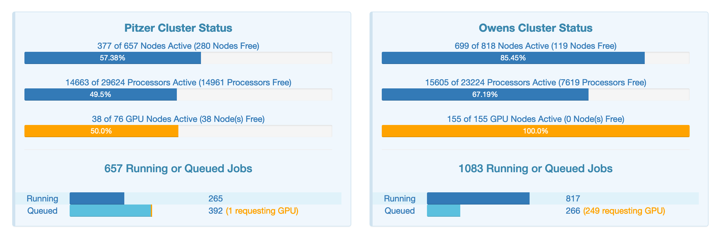
Right now, Pitzer seems the better choice.

For the standard compute nodes the main difference in Owens has 28 cores per node and Pitzer has 40 or 48 cores per node.

Estimating required resources using the scheduler

Although we covered requesting resources from the scheduler earlier, how do we know how much and what type of resources we will need in the first place?

Answer: we don’t. Not until we’ve tried it ourselves at least once. We’ll need to benchmark our job and experiment with it before we know how much it needs in the way of resources.

The most effective way of figuring out how much resources a job needs is to submit a test job, and then ask the scheduler how many resources it used. A good rule of thumb is to ask the scheduler for more time and memory than your job can use. This value is typically two to three times what you think your job will need.

Benchmarking bowtie2-build

Create a job that runs the following command in the same directory as our Drosophila reference genome from earlier.

bowtie2-build Drosophila_melanogaster.BDGP6.\*.toplevel.fa dmel-index

The bowtie2-build command is provided by the bowtie2 module. As a reference, this command could use several gigabytes of memory and up to an hour of compute time, but only 1 cpu in any scenario.

You’ll need to figure out a good amount of resources to ask for for this first “test run”. You might also want to have the scheduler email you to tell you when the job is done.

Do not run jobs on the login nodes

The example above was a small process that can be run on the login node without too much disruption. However, it is good practice to avoid running anything resource intensive on the login nodes. There is a hard limit of 1GB RAM and 20 minutes, anything larger will be automatically stopped.

Here is an example of a job script that would run the process above on a compute node and copy the results back.

#!/bin/bash
#SBATCH --partition=debug
#SBATCH --account=PZSXXXX
   #Give the job a name 
#SBATCH --job-name=bowtie-dros
#SBATCH --time=00:45:00
#SBATCH --nodes=1 --ntasks-per-node=20

set echo
module load bowtie2
cd $SLURM_SUBMIT_DIR
cp Drosophila_melanogaster.BDGP6.*toplevel.fa $TMPDIR
cd $TMPDIR
bowtie2-build Drosophila_melanogaster.BDGP6.*toplevel.fa dros-index
cp *.* $SLURM_SUBMIT_DIR

This job requests 20 cores on one node, which is not needed for this calculation, but if you are unsure about how much memory or how many processors your job will require, it is okay to request more than you need. As you run jobs, you will get more comfortable identifying the amount of resources you need.

cd $SLURM_SUBMIT_DIR

This line ensures we are in the correct starting directory, where the input files are located. If your input files are not in same directory as your job script, you can specify a different location.

cp Drosophila_melanogaster.BDGP6.*toplevel.fa $TMPDIR

Now, we can copy the input file to the compute node, known as $TMPDIR until the job is assigned to a node. We used a wildcard “*” to make the filename more general and the script more flexible. This is good practice so your job scripts can easily be copied and reused for similar jobs.

cd $TMPDIR
bowtie2-build Drosophila_melanogaster.BDGP6.*toplevel.fa dros-index
cp *.* $SLURM_SUBMIT_DIR

Finally, we move the job to the compute node and run the software. All the files will be read and written on the compute node. This makes your job run faster and keeps the job traffic from impacting the network. In the final line, we copy back any output files. I used a very general wildcard to copy everything back, but you can be more specific, based on your job.

A note about memory: Memory (RAM) is allocated based on number of processors requested per node. For example, if you request 14 ppn on Owens, that is half the available processors so your job will receive half the available memory (~64GB). This applies to Owens and Pitzer.

Playing nice in the sandbox

You now have everything you need to run jobs, transfer files, use/install software, and monitor how many resources your jobs are using.

So here are a couple final words to live by:

• Don’t run jobs on the login node, though quick tests are generally fine. A “quick test” is generally anything that uses less than 1GB of memory, and 20 minutes of time. Anything larger will be automatically killed by the system. Remember, the login node is to be shared with other users.

• Compress files before transferring to save file transfer times with large datasets.

• Use a VCS system like git to keep track of your code. Though most systems have some form of backup/archival system, you shouldn’t rely on it for something as key as your research code. The best backup system is one you manage yourself.

• Before submitting a run of jobs, submit one as a test first to make sure everything works.

• The less resources you ask for, the faster your jobs will find a slot in which to run. The more accurate your walltime is, the sooner your job will run.

• You can generally install software yourself, but if you want a shared installation of some kind, it might be a good idea to email OSCHelp@osc.edu.

• Always use the default compilers if possible. Newer compilers are great, but older stuff generally means that your software will still work, even if a newer compiler is loaded.

Final Exercise

We will run the bowtie job in the Job Composer by creating a job from specified path.

• In the Job Composer, select New Job and From Specified Path
• In the new window, enter the path for your job. It should be ` ~username/genome`
• Fill out the rest of the form with the job name, the name of the job script file, cluster, and project code. For this exercise, we will use Owens.
• Select Save You’ll see your job in the composer list. Now, we need to update the job script with your project code and correct file names. Update and save the file and then click the green Submit button. If you see a green bar at the top, it was submitted successfully. If the job runs successfully, you’ll see new files added to your job directory.

Key Points

• The smaller your job, the faster it will schedule.

• Don’t run stuff on the login node.

• Again, don’t run stuff on the login node.

• Don’t be a bad person and run stuff on the login node.